I wrote an article about on how to create an auto-updating Gantt chart in Excel 2010 or 2013. But users of older versions of Microsoft Office might find the instructions difficult to follow.
This article shows you how to do the same thing, but in Excel 2003.
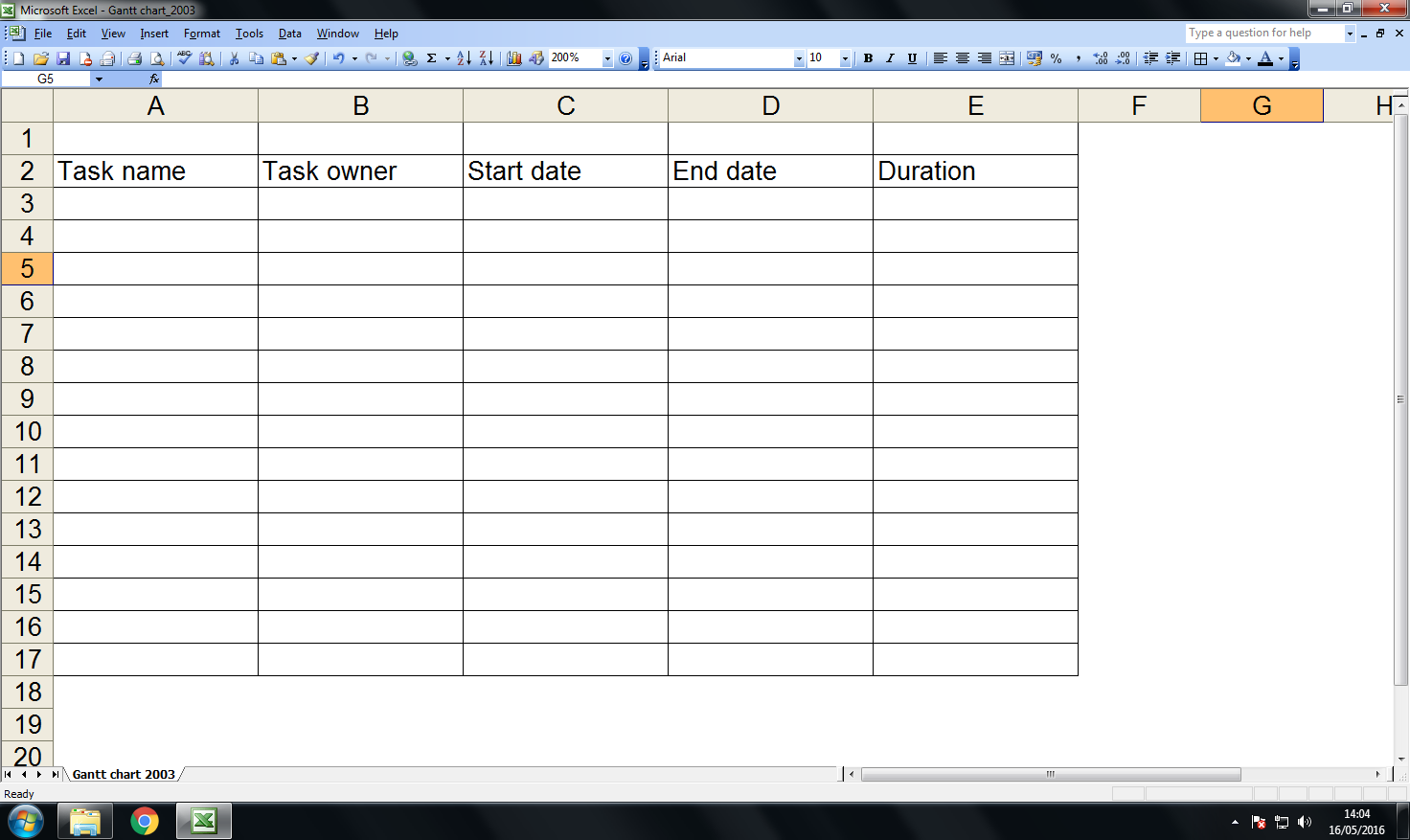
As in the main article, create the table you can see in the screenshot below. For the rest of this walkthrough, I’m going to assume your table is set up like this one. If it isn’t, when I say ‘select cell D3’ — or whatever — you’ll have to work out which cell that should be in your table.
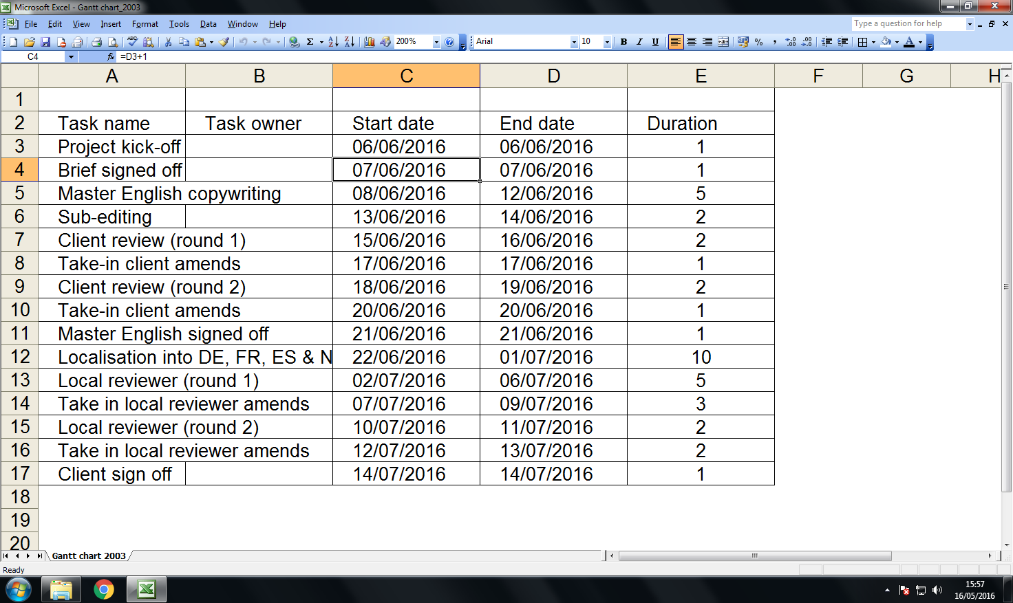
Next populate the table with the details of your project. But hold on, don’t enter all the details manually. This is where we start adding formulas.
Make sure all the cells in the columns headed ‘Start date’ and ‘End date’ are formatted as dates. Enter the start date of your project in the first cell under the header ‘Start date’. In our sample that’s cell C3. No formulas so far; you enter this value manually
Click into cell D3 and enter the formula:
=(C3+E3)-1
This tells Excel that cell the value of D3 is equal to the value of cell C3 plus cell E3 but minus one. You have to subtract one day because the spreadsheet doesn’t understand that the start date itself counts toward the task duration.
Grab the cell D3 and drag down to copy the formula to all the remaining cells in your ‘End date’ column. Click into the ‘Start date’ cell for task two, cell C4. Enter the following formula:
=D3+1
This tells Excel that task two starts the day after task one ends. Now grab the cell with your cursor and drag down to copy that formula to all the remaining cells in the ‘Start date’ column.
3. Add task owners
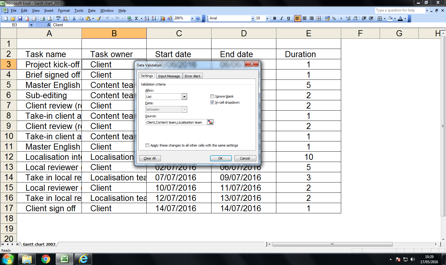
To add task owners, select all the cells in column B of your ‘tasks and dates’ table. With these cells selected, click on the Data menu in the toolbar and select Validation. From the drop-down box labelled Allow, choose the value List.
Ignore the box labelled Data, it will be greyed out. In the box labelled Source, enter the names of the different task owners for your project. For us that’s:
Client,Content team,Localisation team
Each item should be separated by a comma. Make sure that the box labelled In-cell dropbox is ticked, then click ok. Now, when you click into any cell in column B, a drop-down menu containing the values you just entered should appear.
From the drop-down list, select the appropriate task owner for each task in your table.
4. Create week one of the Gantt chart
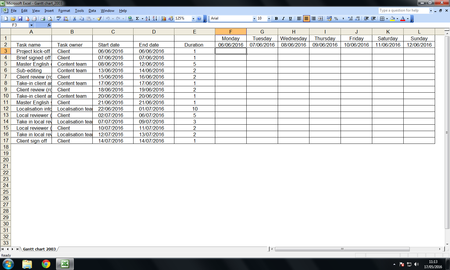
We’ll add week one of the chart and once it’s finished, we’ll copy it to create all the other weeks. Add the cells you can see in columns F to L of the screenshot below.
In row two, don’t just type the dates in, or you’ll have to manually update them every time your project timeline changes. Instead, click into the date cell for Monday and enter the following:
=C3
C3 is the start date of the first task in our table of tasks, so this just synchronises the start dates for the table and the Gantt chart.
Select the date cell for Tuesday, in our case cell G2, and enter the following:
=F2+1
Copy the formula to the remaining cells in row two of your week-one Gantt chart. This tells Excel that the header date for each column is one day later than that of the column to the left of it.
Before we add the formulas that will power our Gantt chart, we need to install an add-in. From the Tools menu, select Add-Ins, then Analysis ToolPak. Click on OK. The “toolpak” will install itself.
Now, click in the first cell in the Gantt chart area of your table. In our sample table, that’s cell F3. Enter the following formula:
=IF(AND(F$2>=$C3,F$2<=$D3),”yes”,”no”)
Press Enter and the word ‘yes’ should appear in the cell F3. For more information about the formula, see step 5 of the main walkthrough. If you get an error message, try deleting and re-typing the quotation marks around the words ‘yes’ and ‘no’.
5. Copy the formula to the rest of your first week
Again, nice and simple — select cell F3 and hover your mouse cursor over the bottom right-hand corner of the cell. When the cursor turns into a black cross, drag down the way to copy the formula into all the other cells in the Monday column of your Gantt chart.
6. Add the formatting
Select the cells in week one of your Gantt chart. Make the text white, so you can’t see it against the white background. On the toolbar, click on the Format menu. Select Conditional Formatting.
In the box that pops up, you want to set condition one as “Cell Value Is equal to yes” (Microsoft’s whacky capitalisation; not mine), as in the screenshot.
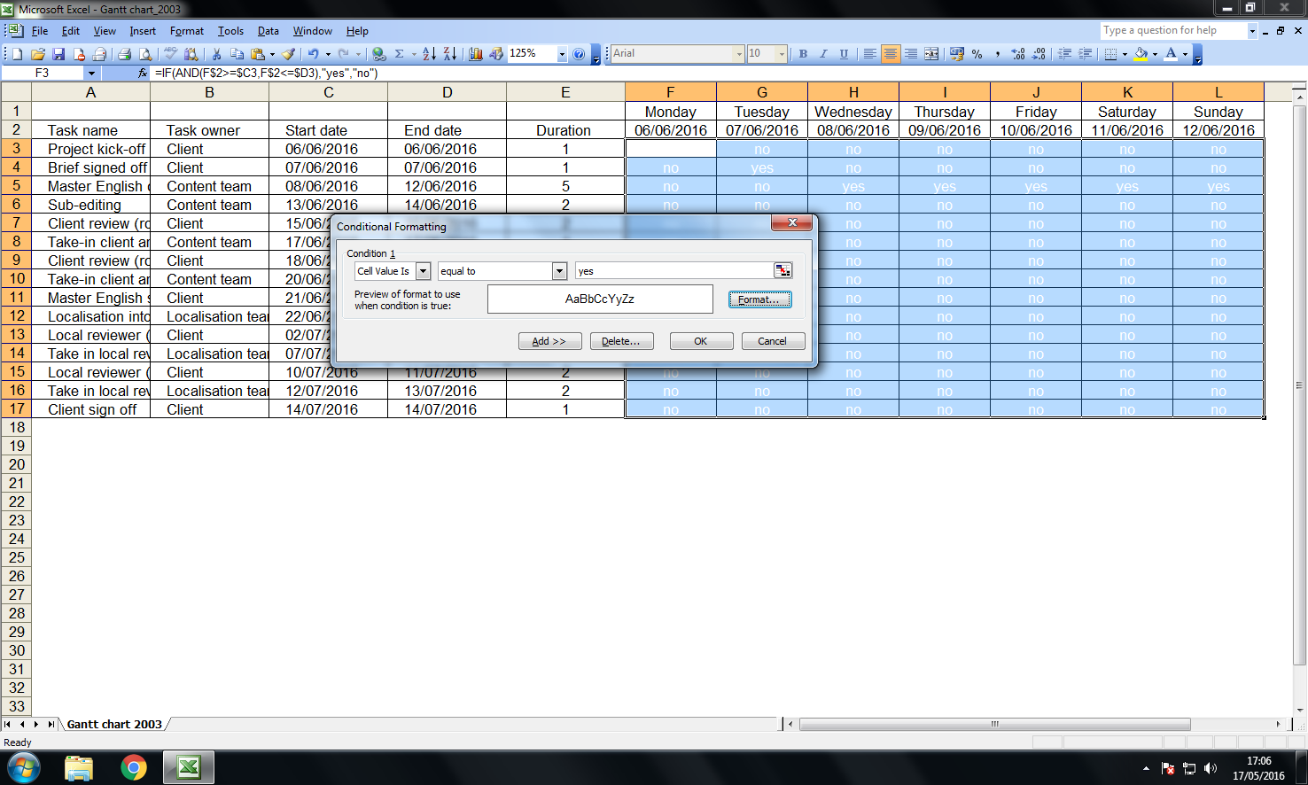
Next click on the button labelled Format. On the tab labelled Font, set the colour of the font as red. Click on the tab labelled Patterns and select the same red as you chose for Font.
To create the full Gantt chart, copy week one and then paste into the empty space to the right of your chart. Repeat until you’ve got enough columns to display all the tasks in your tasks table.
Remember, the date for Monday of week two will be wrong, because you copied it from week one, which was set up to refer to the start date in your table of tasks. You’ll have to manually change it to be Sunday of week one, plus one. In our sample, that would mean entering the formula:
=L2+1
You may have to resize the columns you’ve just copied, in order to be able to see the days and the dates, but otherwise you’re finished and the sheet is ready to use.

