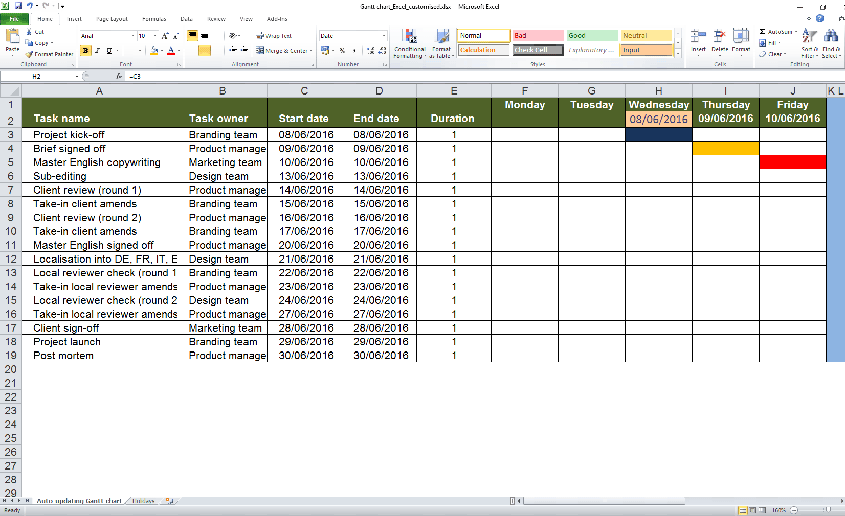
In a previous post, I explained how you can create an auto-updating Gantt chart in Excel. If you work on projects with shifting start dates and task durations, using a chart that updates automatically whenever you change one those variables will save you a lot of time.
But building the sheet can take up to a full day, depending on how familiar you are with Excel. If that’s too long, download the sample worksheet and customise it for your project.
1. Update the list of tasks
Our sample sheet has 15 tasks. Let’s assume your project has 17. Here’s how to add the extra two tasks:
- Delete the sample tasks in column A.
- Delete the task owners in column B.
- Delete the task durations in column E.
Now copy the last two rows of the table, select cell A18, right-click and from the context menu choose Paste. And that’s it, you’ve added two tasks to your table.
If you want to check whether the formulas have been copied, set every task duration to one day. Each task’s start date should be one work day after the end date of the task before.
The only time a task won’t start on the next day, is if the next day is a weekend or one of the UK public holidays listed in the second worksheet, the one named Holidays.
2. Change the task owners
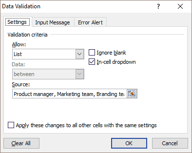 Let’s assume there are four task owners on your project: Product manager, Marketing team, Branding team, Design team.
Select the cells in row B, the one labelled Task owner. From the Data tab on the Ribbon toolbar, click on Data Validation.
From the drop-down list under the word Allow choose the value List. Make sure the box In-cell dropdown is ticked.
In the box labelled Source, enter your list of task owners. Each item should be separated from the next by a comma. In this example:
Product manager, Marketing team, Branding team, Design team
Remember, this bit of the sheet is for humans to read, so make the names meaningful for everyone else who will use the worksheet.
Select cell F3, the first cell in your Gantt chart area. It contains this formula:
IF(AND(F$2>=$C3,F$2<=$D3),IF($B3=”Client”,”Client”,IF($B3=”Content team”,”Content”,IF($B3=”Localisation team”,”Localisation”))),”no”)
Replace the names ot the sample stakeholders with the names of your actual stakeholders. In our example, the formula in cell F3 should now look like this:
=IF(AND(F$2>=$C3,F$2<=$D3),IF($B3=”Product Manager”,”Product”,IF($B3=”Marketing team”,”Marketing”,IF($B3=”Branding team”,”Branding”))),”no”)
This should work fine for your first three stakeholders, but you still need to add “Design team”. Click into cell F3 and add the characters in red, exactly where they are in the formula below.
=IF(AND(F$2>=$C3,F$2<=$D3),IF($B3=”Product manager”,”Product”,IF($B3=”Marketing team”,”Marketing”,IF($B3=”Branding team”,”Branding”,IF($B3=”Design team”,”Design”)))),”no”)
To add even add more task owners, simply repeat this process. Put your mouse in the formula, after the word “Design“, enter a comma and then IF($B3=”New taskowner”,”Taskowner”). Keep doing this, until you’ve added all the teams working on your project.
Once you’ve finished, copy this formula to all the other cells in week one of your Gantt chart.
As an aside, if you wanted to be more efficient, then you could change only the name of the task owner, to which the formula refers. For instance, your original formula could read:
IF($B3=”Client”,”state1″…
For your new project, with its new task owners, you’d simply change this to:
IF($B3=”Design team”,”state1″…
3. Change the conditional formatting
The conditional formatting for week one of the Gantt chart is still set up to respond to the names of the original task owners. We need to change this, or your Gantt chart won’t work.
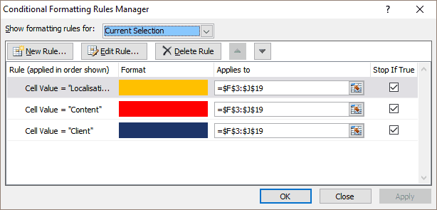
Select week one of the Gantt chart: F3 to J19 (leave the weekend, columns K and L, alone). On the Ribbon toolbar, click on the arrow next to Conditional Formatting and choose Manage Rules.
At the moment, you have three rules: shading cells depending on whether they contain the words “Localisation”, “Content”, or “Client”.
Select the first rule. Click on the button labelled Edit Rule.
The box below will appear. Change =”Localisation” to =”Product” and click OK.
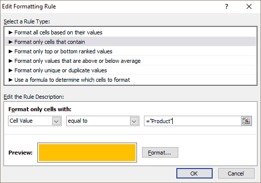
Repeat for the second and third rules, changing to the values to “Marketing” and “Branding” respectively. Finally, you need to add a rule for “Design team”.
In the Conditional Formatting Rules Manager (see above) on the button labelled New Rule.
Select the second option Format only cells that contain.
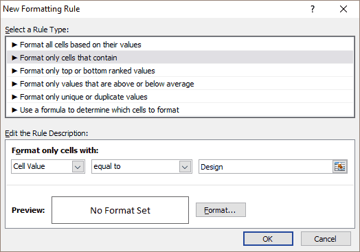
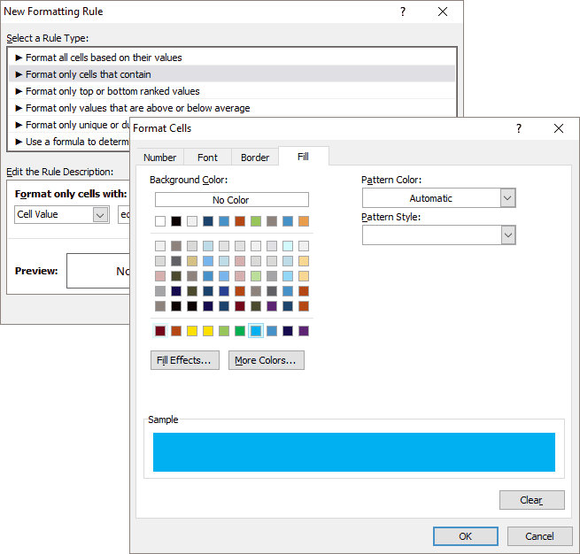
In the screen above, click on the button labelled Format. Set the colour on the tabs Font and Fill, choosing the exact same colour on both tabs.
5. Add additional weeks to your Gantt chart
To add a second week to your Gantt chart cells F1 to L19. Click into cell M1 and paste. Oh dear, everything’s broken. Don’t worry, it’s easy to fix. Copy cell J2 and paste its contents into cell M2.
Select column J by clicking on the letter ‘J’ in the header and copy the entire column. Right-click and from the context menu select Copy.
Select column M. Right-click anywhere in the selected area and from the context menu click on Paste Special. Select the radio button labelled Column widths and click on OK.
To get enough columns to display all your tasks, copy week two — including column headers and the Saturday and Sunday columns — click into cell T1 and paste. Keep doing this until all the tasks in the your table are visible on your Gantt chart.
6. Start projects on a day other than Monday
Starting a project on a day other than Monday is easy. Let’s say your project starts on a Wednesday. Select cells F2 and G2 and delete their contents.
Oops! All of a sudden everything’s broken and your project starts on 1 January 1900. No problem. Click into cell H2, which contains the date for Wednesday. Type =C3 and press Enter.
This links the date for Wednesday, the day on which your project now starts, to the start date in your table of tasks.
7. Protect the sheet
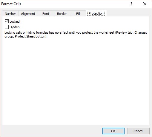
To protect your worksheet, select all cells by clicking on the very top of the left-hand sidebar, in the space between the number 1 and the letter A. Right click one of the selected cells and choose Format Cells. On the Protection tab, ensure that the box labelled Locked is ticked and click OK.
Click anywhere on the sheet to deselect all the sheet’s cell. Now, we have to unlock the cells you want the user to be able to edit. These are:
- All the cells in the first column; the one labelled Task name (A2 to A19 in our worksheet).
- The cell in your table of tasks that contains task one’s start date (C3 in our sample worksheet).
- All the cells in the Task duration column (E3 to E19 in our worksheet).
Select these cells, all together or one at a time. Right click, choose Format Cells from the context menu, and on the Protection tab this time make sure the box labelled Locked is unticked.
Finally, on the tab of the Ribbon toolbar named Review, click on the grid icon above the words Protect Sheet. Click on OK in the box that pops up.
And that’s it. Your worksheet is customised, protected, and ready to use.

