Table of contents
- 1. Create a table of dates
- 2. Populate the table
- 3. Add task owners
- 4. Add week 1 of your Gantt chart
- 5. Now add the formula that will power your Gantt chart
- 6. Copy the formula to the rest of your first week
- 7. Adding the formatting
- 8. Add the extra weeks to your Gantt chart
For a while, when I was working avs a content manager on the HP account at Publicis, we used Microsoft Project. I loved it and so did the rest of the team. But none of our clients used it. We got used to them asking for “something like this, but in Excel”.
So that’s what I created. I didn’t have the patience to manually colour rows of cells, only to change them all when the start date or task durations changed. So I used formulas and conditional formatting to create a sheet that would auto-update if you changed either of those values.
Here’s how you do it.
1. Create a table of dates
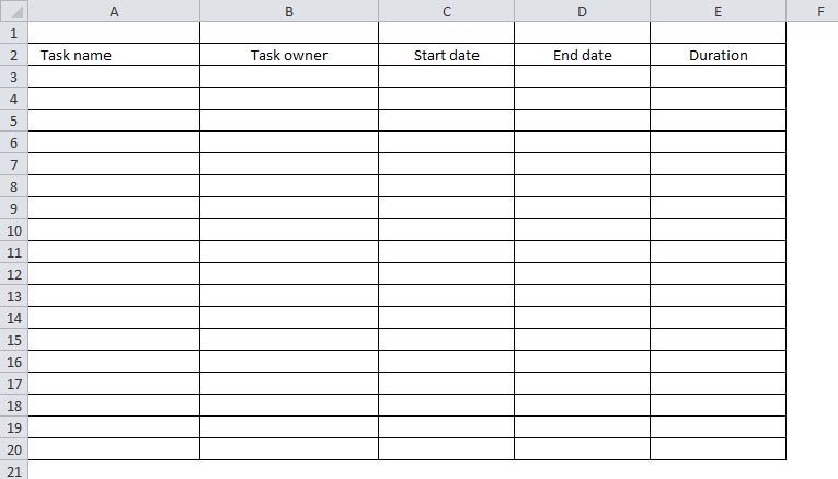
OK, this is the easy bit. In a new spreadsheet, starting from cell A2 (Why A2? We’ll come to that later), re-create the table you can see in the screenshot below.
Break your project down into tasks and fill in the table with the details of those tasks: the task name, start date, end date, and duration. But don’t enter all this information manually.
Click in the first cell in your column labelled ‘Start date’ and enter your project’s start date. Now click in the corresponding cell in the ‘End date’ column and enter this formula (we’re assuming that C3 is the cell containing the start date and E3 contains the task’s duration):
=(C3+E3)-1
This tells the spreadsheet that the end date of the task is equal to the start date plus the duration, minus one day. You have to knock off one day because the spreadsheet isn’t clever enough to understand that the start date itself counts toward the duration of the task.
Now click into the cell corresponding to the next task’s start date (C4, in our example) and enter this formula.
=D3+1
This sets the next task to start one day after previous task finishes.
Now drag and copy both formulas to the other cells in their respective columns. Remember not to copy anything to the first cell in your ‘Start dates’ column: you want to enter that manually.
For now, start task one on a Monday. To find out how to start on a day other than Monday, see step 5 in this post. Don’t populate the task owner yet, that’s the next step.
Lastly, in column E, add the duration in days of each task.
3. Add task owners

When we automate the Gantt chart, it’s going to be important that task owners are assigned properly. For this reason, we’ll restrict the values users can enter here.
In the Ribbon menu on Microsoft Excel click on the Data tab (Using a version of Excel that has menus not tabs? Here’s a tutorial for anyone using Excel 2003 or earlier) . Select the cells in the column headed ‘Task owner’ and, in the Ribbon, click on the drop-down arrow next to the words Data validation. Choose the menu item labelled ‘Data validation…‘.
Click on the box labelled Allow and from the drop-down menu select List. In the box labelled Data: enter the names of your task owners, separated by a comma. Our task owners are the client, the content team and the localisation team, so we enter:
Client,Content team,Localisation team
These values will now appear as a drop-down list in the cells you highlighted. Everyone has to choose one of these when defining a task owner.
4. Add week 1 of your Gantt chart
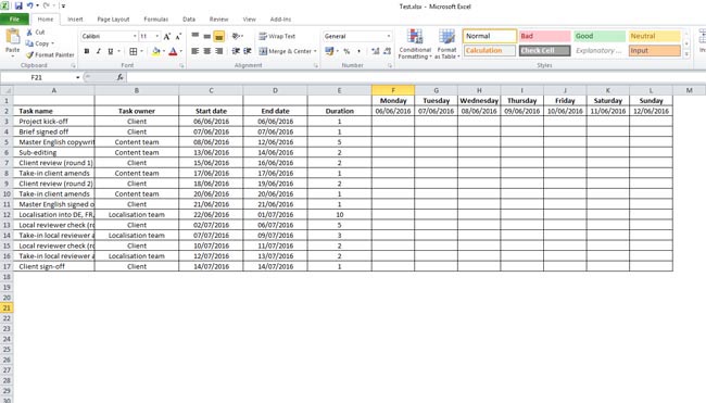
Now the table’s done, let’s start the Gantt chart. In the cell F1 type ‘Monday’, then fill in the days of the week in cells G1, H1 and so on, until you have enough columns for one full week. Select cells F2 to L2, right click, choose Format Cells from the context menu and format as a date.
Now select F2, type the equals sign and then select the cell containing the start date of your first task; in our sample sheet that’s C3. Cell F2 now contains the formula =C3. Select cell G2, type the equals sign and then click on cell F2 and enter +1. G2 will now display the date of your start date plus one. Do the same for all of the cells from F2 to L2. When you’re done, each cell in the series should display the date of the cell to the left of it, plus one.
5. Now add the formula that will power your Gantt chart
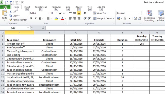
To start making the Gantt chart, click in the first blank cell in your ‘monday’ column. In our sample worksheet that’s cell F3. Enter the following formula:
=IF(AND(F$2>=$C3,F$2<=$D3),”yes”,”no”)
It looks complicated, but it isn’t. All it says is: “if the value of F2 (the column header cell containing the day’s date) is greater than or equal to C3 (the task’s start date) and equal to or less than D3 (the finish date) the cell containing this formula should display the word “yes” otherwise it should display “no”. As you can see, in our example the cell F3 displays the word ‘yes’.
6. Copy the formula to the rest of your first week
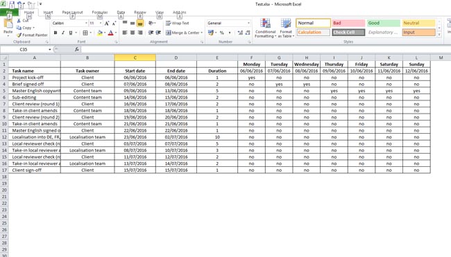
Select cell F3. Hover your cursor over its bottom right corner. When the cursor turns into a black cross, grab the cell and drag downward until the formula has been copied to all the cells in the first column of your Gantt chart. All the cells except F3 should contain the word ‘no’. Now select the ‘Monday’ column and drag your cursor to copy the formula into all the other cells in week one.
7. Adding the formatting

We could just stop here. The mechanics of the Gantt chart are now in place. If you change the duration of a task, for every day you add the relevant column will display the word ‘yes’; and the first yes in the next row now shows up on the day after the previous task’s new end date.
But scanning rows and columns for the words ‘yes’ and ‘no’ isn’t a good user experience. So let’s add some formatting. Select cells F4 to L15 and set the text colour to white. The text in the cells will no longer be visible.

With the cells still selected, on your Home tab, click on the drop-down arrow next to Conditional Formatting. Choose Highlight Cell Rules and then Equal to. In the box that appears, under the heading Format cells that are equal to, enter the word ‘yes’.
In the drop-down box that appears after the word “with”, choose Custom Format… On the tab labelled Font, click on the drop-down box under the word Color and select More Colors… Click on the tab Custom and enter the values 255 for red and 0 for blue and green. Close the Font dialog box, go to the tab Fill and repeat the process, to make the background the same red as the text.
Now every time you update a task duration, the relevant cells in your Gantt chart will turn red. Congratulations, you have an auto-updating Gantt chart.
8. Add the extra weeks to your Gantt chart
The only thing remaining is to extend your Gantt chart so that there are enough columns to display every task in your table of tasks and dates. This is really easy. Select week one and copy it. Now paste the data you’ve just copied into the space immediately to the right of week one.
It looks horrible doesn’t it. Everything’s broken. Don’t worry, that’s just because the date for the second Monday in your chart is wrong. Click in the date cell for the Monday of the second week and enter the equals sign, now click on the date cell for the previous Sunday and then add +1.
So in our sample file, the contents of this cell now read:
=L2+1
Your week-two columns may also be too narrow. To fix this, select a column in week one, right click and choose Copy from the context menu. Now select all the columns in week two by clicking on the column headers and dragging.
Right click and in the context menu, look for the words Paste Special… If you hover your cursor over them, theses words will open a sub menu. Don’t click on the sub menu, instead click on the words Paste Special in the main context menu. In the box that pops up, choose Column Widths.
And that’s it. To finish your chart, copy the columns for week two in your Gantt chart and paste them into the empty space just to the right of week two. Keep repeating this process until you have enough columns to display every task in your table of tasks.
What’s coming in part two
In part two of this post, we’ll look at how to stop the chart scheduling tasks on weekends, local holidays or just days when your team or your client won’t be available.
We’ll also customise the the bars on the Gantt chart to change colour depending on who the task owner is. And we’ll see how to get around the limitation of having to start projects on a Monday.
